Scikit-learn integration
This page shows how to use chemotools in combination with scikit-learn. The following topics are covered:
- Working with single spectra
- Working with pipelines
- Working with pandas DataFrames
- Persisting your models
Working with single spectra
Preprocessing techniques in scikit-learn are primarily designed to work with 2D arrays, where each row represents a sample and each column represents a feature (i.e., matrices). However, in spectroscopy, single spectra are often of interest, which are represented as 1D arrays (i.e., vectors). Below there is an example of a single spectrum:
array([0.484434, 0.485629, 0.488754, 0.491942, 0.489923, 0.492869,
        0.497285, 0.501567, 0.500027, 0.50265 ])
To apply scikit-learn and chemotools techniques to single spectra, they need to be reshaped into 2D arrays (i.e., a matrix with one row). To achieve this, you can use the following code that reshapes a 1D array into a 2D array with a single row:
import numpy as np
from chemotools.scatter import MultiplicativeScatterCorrection

msc = MultiplicativeScatterCorrection()
spectra_msc = msc.fit_transform(spectra.reshape(1, -1))
The .reshape(1, -1) method is applied to the 1D array spectra, which is converted into a 2D array with a single row. An example of the output of the .reshape(1, -1) method is shown below:
array([[0.484434, 0.485629, 0.488754, 0.491942, 0.489923, 0.492869,
         0.497285, 0.501567, 0.500027, 0.50265 ]])
The output of the
.reshape(1, -1)method is a 2D array with a single row. This is the format thatscikit-learnandchemotoolspreprocessing techniques expect as input.
Working with pipelines
Pipelines are becoming increasingly popular in machine learning workflows. In essence, pipelines are a sequence of connected data processing steps, where the output of one step is the input of the next. They are very useful for:
- automating complex workflows,
- improving efficiency,
- reducing errors in data processing and analysis and
- simplifying model persistence and deployment.
All preprocessing techniques in chemotools are compatible with scikit-learn and can be used in pipelines. As an example, we will study the case where we would like to apply the following preprocessing techniques to our spectra:
- Whittaker smoothing
- ArPls baseline correction
- Mean centering
- PLS regression
In a traditional workflow, would apply each preprocessing technique individually to the spectra as shown in the image below:
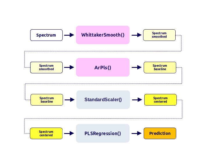
The code to perform this workflow would look like this:
from sklearn.cross_decomposition import PLSRegression
from sklearn.preprocessing import StandardScaler

from chemotools.baseline import ArPls
from chemotools.smooth import WhittakerSmooth

# Whittaker smoothing
spectra_smoothed = WhittakerSmooth().fit_transform(spectra)

# ArPls baseline correction
spectra_baseline = ArPls().fit_transform(spectra_smoothed)

# Mean centering
spectra_centered = StandardScaler(with_mean=True, with_std=False).fit_transform(spectra_baseline)

# PLS regression
pls = PLSRegression(n_components=2)
pls.fit(spectra_centered, reference)
prediction = pls.predict(spectra_centered)
This is a tedious and error-prone workflow, especially when the number of preprocessing steps increases. In addition, persisting the model and deploying it to a production environment is not straightforward, as each preprocessing step needs to be persisted and deployed individually.
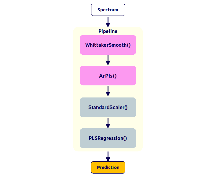
A better approach is to use a pipeline, which automates the workflow and reduces the risk of errors. The figure below shows the same workflow as above, but using a pipeline:
The code to perform this workflow would look like this:
from sklearn.cross_decomposition import PLSRegression
from sklearn.pipeline import make_pipeline
from sklearn.preprocessing import StandardScaler

from chemotools.baseline import ArPls
from chemotools.smooth import WhittakerSmooth

pipeline = make_pipeline(
    WhittakerSmooth(),
    ArPls(),
    StandardScaler(with_std=False),
    PLSRegression(n_components=2)
)
Now the pipeline can be visualized, which will show the sequence of preprocessing techniques that will be applied in the pipeline and their parameters:
Once the pipeline is created, it can be used to fit and transform the spectra and to make predictions:
prediction = pipeline.fit(spectra, reference).predict(spectra)
The preprocessed spectra produced by the previous pipeline is shown in the figure below.
Notice that in the traditional workflow, the different preprocessing objects had to be persisted individually. In the pipeline workflow, the entire pipeline can be persisted and deployed to a production environment. See the Persisting your models section for more information.
Working with DataFrames (🐼 and 🐻❄️ )
For the pandas.DataFrame and polars.DataFrame lovers. By default, all scikit-learn and chemotools transformers output numpy.ndarray. However, now it is possible to configure your chemotools preprocessing methods to produce either a pandas.DataFrame or a polars.DataFrame objects as output. This is possible after implementing the new set_output() API from scikit-learn (>= 1.2.2 for pandas and >= 1.4.0 for polars)(documentation). The same API implemented in other scikit-learn preprocessing methods like the StandardScaler() is now available for the chemotools transformers.
From version 0.1.3, the
set_output()is available for allchemotoolsfunctions!
Below there are two examples of how to use this new API:
Example 1: Using the set_output() API with a single preprocessing method
1. Load your spectral data as a pandas.DataFrame.
First load your spectral data. In this case we assume a file called spectra.csv where each row represents a spectrum and each column represents a wavenumbers.
import pandas as pd
from chemotools.baseline import AirPls

# Load your data as a pandas DataFrame
spectra = pd.read_csv('data/spectra.csv', index_col=0)
The spectra variable is a pandas.DataFrame object with the indices representing the sample names and the columns representing the wavenumbers. The first 5 rows of the spectra DataFrame look like this:
| 900.0 | 901.0 | 903.0 | 904.0 | 905.0 | 906.0 | 908.0 | 909.0 | 910.0 | |
|---|---|---|---|---|---|---|---|---|---|
| 0 | 0.246749 | 0.268549 | 0.279464 | 0.280701 | 0.292982 | 0.288912 | 0.297167 | 0.310435 | 0.325145 |
| 1 | 0.235092 | 0.249278 | 0.25094 | 0.251326 | 0.266078 | 0.263885 | 0.279901 | 0.295895 | 0.297663 |
| 2 | 0.227894 | 0.223541 | 0.226005 | 0.23621 | 0.249276 | 0.26032 | 0.258642 | 0.282584 | 0.285163 |
| 3 | 0.204115 | 0.213624 | 0.220228 | 0.222264 | 0.225996 | 0.232336 | 0.235273 | 0.261938 | 0.26663 |
| 4 | 0.195615 | 0.195829 | 0.203789 | 0.220114 | 0.233223 | 0.240248 | 0.246378 | 0.261398 | 0.267355 |
2. Create a chemotools preprocessing object and set the output to pandas.
Next, we create the AirPls object and set the output to pandas.
# Create an AirPLS object and set the output to pandas
airpls = AirPls().set_output(transform='pandas')
The set_output() method accepts the following arguments:
transform: The output format. Can be'pandas'or'default'(the default format will output anumpy.ndarray).
If you wanted to set the output to
polarsyou would usetransform='polars'in theset_output()method (AirPLS().set_output(transform='polars')).
3. Fit and transform the spectra
# Fit and transform the spectra
spectra_airpls = airpls.fit_transform(spectra)
The output of the fit_transform() method is now a pandas.DataFrame object.
Notice that by default the indices and the columns of the input data are not maintained to the output, and the
spectra_airplsDataFrame has default indices and columns (see example below).
The spectra_airpls DataFrame has the following structure:
| x0 | x1 | x2 | x3 | x4 | x5 | x6 | x7 | x8 | x9 | |
|---|---|---|---|---|---|---|---|---|---|---|
| 0 | 0.210838 | 0.213002 | 0.217275 | 0.222833 | 0.229342 | 0.236683 | 0.245315 | 0.254254 | 0.263244 | 0.272121 |
| 1 | 0.219816 | 0.220637 | 0.223478 | 0.227481 | 0.233518 | 0.240035 | 0.247666 | 0.256066 | 0.264704 | 0.273879 |
| 2 | 0.220096 | 0.221503 | 0.224515 | 0.22905 | 0.23486 | 0.242032 | 0.250077 | 0.25948 | 0.268111 | 0.276561 |
| 3 | 0.211932 | 0.213675 | 0.216953 | 0.222211 | 0.22891 | 0.235941 | 0.243654 | 0.252518 | 0.261452 | 0.270276 |
| 4 | 0.212528 | 0.21408 | 0.217522 | 0.222005 | 0.228657 | 0.236576 | 0.244935 | 0.253593 | 0.262239 | 0.271826 |
Example 2: Using the set_output() API with a pipeline
Similarly, the set_output() API can be used with pipelines. The following code shows how to create a pipeline that performs:
- Multiplicative scatter correction
- Standard scaling
import pandas as pd
from sklearn.pipeline import make_pipeline
from sklearn.preprocessing import StandardScaler
from chemotools.scatter import MultiplicativeScatterCorrection

pipeline = make_pipeline(MultiplicativeScatterCorrection(),StandardScaler())
pipeline.set_output(transform="pandas")

output = pipeline.fit_transform(spectra)
If you wanted to set the output to
polarsyou would usetransform='polars'in theset_output()method (pipeline.set_output(transform='polars')).
Persisting your models
In the previous sections, we saw how to use chemotools in combination with scikit-learn to preprocess your data and make predictions. However, in a real-world scenario, you would like to persist your preprocessing pipelines and models to deploy it to a production environment. In this section, we will show two ways to persist your models:
- Using
pickle - Using
joblib
For this section, we will use the following fit pipeline as an example:
from chemotools.scatter import MultiplicativeScatterCorrection
from chemotools.baseline import AirPls
from sklearn.cross_decomposition import PLSRegression
from sklearn.pipeline import make_pipeline
from sklearn.preprocessing import StandardScaler

# create pipeline
pipeline = make_pipeline(
    MultiplicativeScatterCorrection(),
    AirPls(),
    StandardScaler(with_std=False),
    PLSRegression(n_components=2)
)

# fit pipeline
pipeline.fit(spectra, reference)
Using pickle
pickle is a Python module that implements a binary protocol for serializing and de-serializing a Python object structure. It is a standard module that comes with the Python installation. The following code shows how to persist a scikit-learn model using pickle:
Notice that the
picklemodule is not secure against erroneous or maliciously constructed data. Never unpickle data received from an untrusted or unauthenticated source.
import pickle

# persist model
filename = 'model.pkl'

with open(filename, 'wb') as file:
    pickle.dump(pipeline, file)

# load model
with open(filename, 'rb') as file:
    pipeline = pickle.load(file)
Using joblib
joblib is a Python module that provides utilities for saving and loading Python objects that make use of NumPy data structures, efficiently. It is not part of the standard Python installation, but it can be installed using pip. The following code shows how to persist a scikit-learn model using joblib:
from joblib import dump, load

# persist model
filename = 'model.joblib'

with open(filename, 'wb') as file:
    dump(pipeline, file)

# load model
with open(filename, 'rb') as file:
    pipeline = load(file)